What is linearity?

In this small blog article, we would like to explain the parameter “Linearity” for an analytical method validation, its importance, and how it is calculated.

Mathematically speaking, linearity is a function of values that can be graphically represented as a straight line. Similarly, as per the method validation ICH Q2(R1) guideline, the linearity of an analytical method can be explained as its capability to show “results that are directly proportional to the concentration of the analyte in the sample”.

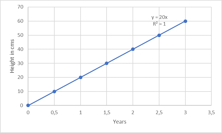
Linearity is often measured within a given range. For example, consider a plant that grows exactly 10 cm every 6 months for 3 years, the growth can be said to be linear for the 3 years.

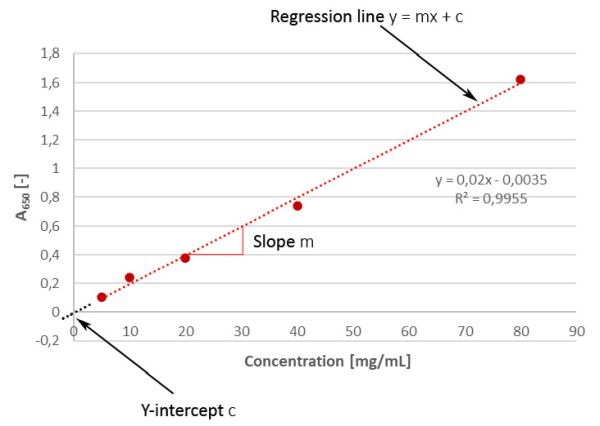
Unfortunately, the analytical response of a method is not always so distinctively linear as in the case of the growth of trees (example above). An example from the analytical lab is e.g. the photometric protein determination according to Markwell: the more protein is present in the solution (i.e. the higher the concentration, variable "x"), the stronger is the developing blue colour (i.e. the measurement signal, here: absorbance at 650 nm, variable "y"). In this context, y is known as the dependent variable.

Regarding analytical methods of drugs and active ingredients, the linearity of a signal can either be the relationship between the analyte’s signal and the analyte’s concentration in the calibration sample or in the sample matrix. The latter is more important because if the analyte’s signal within the sample is linear, it almost certain that it will also be the case in the calibration samples too. However, the same cannot be said for the opposite partly because of the matrix effect. A matrix effect is the influence caused by the other components of the sample to the expected response without the substance to be analyzed (e.g. formulation buffer). In case where the data are not linear, they might be mathematically transformed, e.g. applying logarithms but in some cases like in immunoassays no transformation won’t work at all. This is easy to understand for an ELISA if you consider the underlying principle of the method: a defined number of capture antibodies are bound in each well, which in turn can only bind a certain number of target proteins. This works well (i.e. there is a linear relationship) as long as free binding sites are still available. As soon as all binding sites are occupied, differences between different protein concentrations can’t be differentiated any longer due to the saturation effect!

Linearity is important for the analysis of the analyte’s concentration within a defined range. A defined range is important because for each drug the content of the active ingredient as well as the content of potential impurities is not always exactly identical from batch to batch, but can vary slightly, which is why concentrations above and below the respective expected value must also be determined correctly. As per the method validation ICH Q2(R1) guideline, linearity of a given response must be evaluated using at least a minimum of 5 concentrations of the analyte (multi-point calibration) and the data must be statistically analyzed, e.g. by performing regression analysis using the method of the least squares. To do this, the concentrations of the analyte are plotted on the x-axis against the measured absorbance on the y-axis and a regression line is drawn through the points. The application of least squares means that the "best" line is used for this purpose. The results are required to be represented in terms of the correlation coefficient R, Y-intercept, slope of the regression line and the residual sum of the squares in addition to graphical plotting. There are also a few brief words on residual analysis in the update at the end of this article. In a linear regression line y = mx + c, the regression coefficient is the constant “m” that represents the rate of change of one variable “y” as a function of change in the other “x” (this means for our example above: how much stronger / weaker does the blue colour, measured as absorbance, will become when the concentration of the analyte changes?), while “c” is the Y-intercept. In simple terms, m is the slope and c is the ordinate intersection.

But what do these two parameters like to tell us?

• If the regression line doesn’t pass through the origin (which is actually more or less almost always the case), i.e. we have a positive y-value at a concentration of 0, it provides us an indication of a constant systematic error (offset). In practical terms, this is the blank value, which is subtracted for correction.
• The slope, on the other hand, gives us information about the sensitivity of the method (à “calibration sensitivity”). It is easy to see that a steeper (i.e. greater) slope is associated with greater sensitivity, since it enables the discrimination of small differences in concentration. If, on the other hand, the slope is quite flat, small differences in concentration can’t be detected very well.

While regression tells us something about the relationship between the two variables, the correlation coefficient or coefficient of determination tells us about the strength of that relationship. For a linear data set, calculation of the Pearson’s correlation coefficient R must prove to be sufficient. This coefficient is a value without unit telling us something about the degree of a linear relationship between two variables. If there is a perfect linear relationship, it has a value of 1. In case of a value being less than 0.95, it may either be a result of a broad spreading during measurement or due to a non-linear correlation. Often, the coefficient of determination (R²) is used, which is just the square of it, but which is a sharper criterion than the correlation coefficient due to squaring (see: R = 0.99 à R² = 0.98). For most methods used, at least an R² ≥ 0.98 can be achieved, but there is no general regulatory required value that must be reached as minimum level for a good correlation, although the German ZLG Aide mémoire AiM 07123101 mentions a correlation coefficient R of usually > 0.99. According to Patric U.B. Vogel's trending booklet, R²-values between 0.90 - 0.99 are common indicators of a strong correlation in analytics, depending on the analytical method used. It is easy to understand that for well standardized chemical methods such as HPLC, calibration curves with an R² of ≥ 0.99 can be obtained, while for some biological test systems R² can be significantly lower, which is simply due to the inherent natural increased variability of the biological test system compared to chemical HPLC.

It is mandatory for purity and assay methods (assays include content and potency determinations) to perform linearity studies for the validation of these methods. Linearity studies are important because they define the range of the method within which the results are obtained accurately and precisely. In case of impurities with very small amounts to be quantified, the limit of quantification (LOQ) needs to be evaluated. For the LOQ, trueness is also mandatory. Evaluating linearity near the LOQ (combined with repeatability and given specificity) can be used to infer trueness.

 

To summarize, linearity is one major aspect in the method validation procedure of assays and quantitative impurity tests. It provides to assess the range of concentrations for which the method can reliably function. For validation, multi-point calibration techniques are accepted, while single point calibrations are not. In case of a non-linear data set, higher order equations might be transformed, or the data must be accepted as they are while demonstrating a clear relation between analyte concentration and response.

 

Update: Residual analysis

As mentioned above, the regression line is drawn according to the least squares method. Thus, it is a compensation line and the individual values on which it is based all deviate a little bit. Sometimes upwards, sometimes downwards. Let’s illustrate this with an example. We perform a protein determination and get the following data set:

Conc. [mg/mL]	Absorbance  A650 [-]		Residual
	measured	calculated
5	0.103	0.096	0.007
10	0.240	0.196	0.044
20	0.377	0.396	-0.019
40	0.736	0.796	-0.060
80	1.624	1.595	0.029
			Σ = 0

Here, the "calculated" values correspond to the values that we would obtain with the help of the equation of the regression line, i.e. the ideal values of our regression line. If we then compare (i.e. subtract) the measured value with the calculated value, we obtain the residual, i.e. the respective deviation. Graphically, a residual plot of such a residual analysis looks like this:

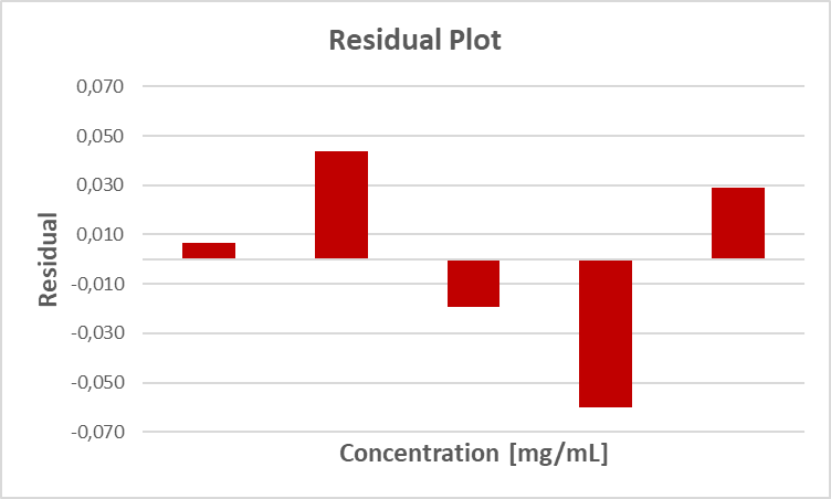
How much significance is in this figure and in such a residual analysis in general, remains to be seen...

References

[1] International Council for Harmonisation of Technical Requirements for Pharmaceuticals for Human Use (ICH) (2023) “Validation of Analytical Procedures“ Q2(R2)
[2] Markwell MA, Haas SM, Bieber LL, Tolbert NE. A modification of the Lowry procedure to simplify protein determination in membrane and lipoprotein samples. Anal Biochem. 1978 Jun 15;87(1):206-10.
[3] National Health Surveillance Agency (ANVISA) (2017) Resolution of the collegiate board RDC No. 166
[4] Zentralstelle der Länder für Gesundheitsschutz bei Arzneimitteln und Medizinprodukten (2017) „Inspektion von analytischer Validierung und Methodentransfer“ (AiM 07123101)
[5] Vogel P.U.B. (2020). Trending in der pharmazeutischen Industrie, Springer Spektrum, Wiesbaden, ISBN: 978-3-658-32206-9