Linear versus non-linear regression: What should be considered?
In any quantification method of a drug or its active ingredient, the linearity of the calibration line is a crucial criterion for the correctness of the values. The measured values should, in the best case, be directly proportional to the concentration of the analyte in the sample. Most methods have their limits; therefore, you often narrow the measurable range (linear range).
According to the ICH Q2(R2) Method Validation Guideline, the linear response (linearity) must be demonstrated within the reportable range applying the method of least squares to calculate the regression line. It is mandatory to avoid enforcing a linear regression on data being non-linear. If a curve can be obtained when plotting the concentration against the measured values, a more detailed regression analysis should be considered.
Linear or non-linear: correlation coefficients help to decide
In case of a shallow curve, the decision as to whether linear regression can be applied, belongs to the analyst. A possible aid could be the calculation of two correlation coefficients (R). One could argue that calculation of a Pearson coefficient should be sufficient, but Pearson’s correlation coefficient only considers linear relationships. For example, if the coefficient value is significantly lower than 0.95, it may either be a result of a measurement value’s scatter being too high or due to a non-linear correlation. Certainty can be obtained by calculating Spearman’s correlation coefficient. This method respects both linear and non-linear correlations. A higher value for the Spearman’s coefficient compared to Pearson’s coefficient points towards a non-linear correlation. If both correlation coefficients are nearly identical, a linear correlation exists.
Transformation of the raw data
For a non-linear dependence, the ICH Q2(R2) guideline proposes a mathematical transformation of the raw data to provide a suitable linear regression. How can it be performed?
In the given example, we have generated hypothetical values that follow a second order polynomial function (y = ax2 + bx + c). The graphical representation is shown in the first figure (blue values).
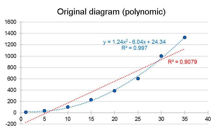
It can be clearly seen, that no linear regression can be applied. If tried anyways, a coefficient of determination (R2) value of 0.908 is obtained. On the other hand, a polynomial function can clearly be inserted on the dataset (blue line). A simple way of bringing the polynomial function into a linear dependence is the so-called "ladder of powers". Depending on the type of curve, the ladder of powers can be used to determine the changes that must be applied on x or y variables to reach a linear dependence (refer to the following figure):
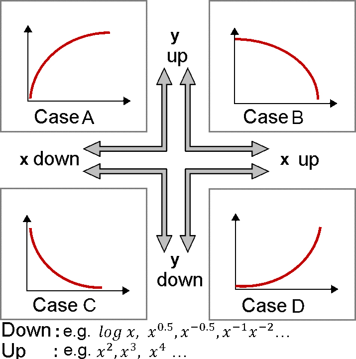
If, as in the example, a rising curve is observed ("Case D" in the figure above), then the x-variable can be raised to a power of 2 (square) or 3 (cube). Another approach would be to lower the y variable by, for example, a factor of logarithm or root function, to gradually approach linearity. In the provided example the root function was used on the y variables (= y0.5) and the following result was calculated:
![]()
After performance of the corresponding mathematical transformations, linear regression can be applied on the newly obtained x and y values and the coefficient of determination (R2) can be calculated. In this example, a good linear relationship with a coefficient of determination value of 0.993 was obtained. New data that are to be analysed using the transformed linear regression must be subjected to the same mathematical transformation before analysis. In our example, all newly measured “Y” values must be rooted. Afterwards, the obtained values can be used for the regression equation and resolved to x.