Where does linearity end - is there an "upper limit"?

Introduction

Although this time it’s not about pharmaceutical method validation¹, I’d like to take up an interesting question about the upper limit of linearity. We’ve got the following topic: For the performance of real-time polymerase chain reactions (RT-PCR) to detect SARS-CoV-2, the comparability of 2 thermal cyclers should be determined. For this purpose, the Ct values of the two thermal cyclers (let's call them A and B) were plotted against each other at different sample concentrations. 

 

Some background 

To understand the Ct value (Ct = cycle threshold), it’s important to bear in mind the reaction principle of PCR. In the presence of a primer, the enzyme DNA polymerase extends single-stranded DNA to form a double strand. Subsequently, this double strand is separated by a denaturation step allowing the primers to bind again to both new single strands and to be extended once more to form new double strands. As this process takes place in many successive cycles, a previously small amount of DNA is exponentially amplified in this way. Since the newly synthesized products of the previous cycles serve as starting materials for the subsequent cycles, this is referred to as a chain reaction. Since in our case it's not DNA but RNA that is present, an upstream reverse transcription takes place to convert RNA into DNA and thus to enable the analysis of RNA viruses.

In an RT-PCR, the Ct value denotes the amplification cycle at which the reaction described above enters the exponential phase and thus exceeds a threshold (mathematically, this was already the case previously, but the reaction was not yet detectable, thus being below the threshold).

The Ct value is therefore a measure of - in our example - the RNA concentration of the SARS-CoV-2 virus present in the sample. A low Ct value correlates with a higher RNA concentration, as a lower number of amplification cycles is necessary for detection compared to a higher Ct value, where more cycles had to be run because the initial RNA concentration in the sample was significantly lower.   

 

Back to the example and the question

The plot of the Ct values of the two thermal cyclers looked like this:

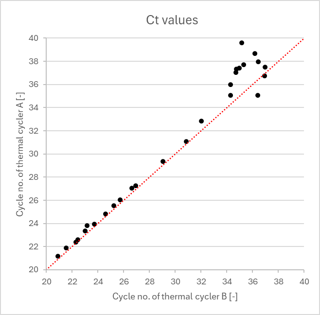
The closer the individual points are to the straight line, the more similar the sample results are for both thermal cyclers. However, it’s noticeable that the values start to scatter from a Ct value of approx. > 34.

It's easy to understand that the less virus material is in the initial sample, the greater the scatter, because the probability decreases that exactly the same amount of RNA could be obtained for both thermal cyclers during pipetting. For this reason, a comparison of the two thermal cyclers only makes sense in the linear range.

This leads to the question: Where does the linear range of the method end, what’s the "upper limit of linearity"? How can we determine this objectively? 

 

Possible solutions

In order not to successively exclude individual points starting from the upper end of the regression line and then check at which point the correlation coefficient R gets closest to 1, but to dive to the bottom of the question more objectively, there are various statistical methods that can be used, such as the calculation of the relative response (factor) or residual analysis. The latter also includes more in-depth statistical techniques such as the determination of D values (Cooks Distance) or H values (Hat Values). There are also other ways of evaluating linearity but listing them here would exceed the scope of this blog article. The use of linearity tests, such as those used to check calibration lines, makes no sense in this example.

Accordingly, the relative response and the residual analysis for our example to determine the upper limit of linearity are presented below.

Since we’ve plotted the Ct values of thermal cycler A against B, the Ct values of thermal cycler A act as y values and those of B as x values. The relative response is calculated as y/x, for the residual we subtract y-x.

Ct value themal cycler B [-] (x [-])	Ct value themal cycler A [-] (y [-])	Relative Response [-]	Residual [-]
20.91	21.19	1.01	0.28
21.53	21.89	1.02	0.36
22.29	22.38	1.00	0.09
22.44	22.60	1.01	0.16
23.03	23.37	1.01	0.34
23.16	23.80	1.03	0.64
23.73	23.93	1.01	0.20
24.60	24.81	1.01	0.21
25.23	25.55	1.01	0.32
25.73	26.06	1.01	0.32
26.63	27.04	1.02	0.41
26.93	27.28	1.01	0.35
29.05	29.35	1.01	0.30
30.88	31.07	1.01	0.19
32.02	32.83	1.03	0.81
34.29	35.97	1.05	1.68
34.30	35.08	1.02	0.78
34.73	37.06	1.07	2.33
34.77	37.34	1.07	2.57
34.97	37.41	1.07	2.44
35.18	39.58	1.13	4.40
35.33	37.69	1.07	2.36
36.19	38.68	1.07	2.49
36.19	40.31	1.11	4.12
36.42	35.08	0.96	-1.34
36.45	37.98	1.04	1.53
36.93	36.73	0.99	-0.20
36.97	37.49	1.04	0.52

Afterwards, we calculate the mean of the relative response (here: 1.031, considering all values, which may well be questioned) and define corresponding limits (here: exemplarily ± 3% of the mean, i.e. 1.000 & 1.062). The basis on which the limits are defined, as well as the question of whether all values should be used for the calculation of the mean or whether individual values should be previously excluded based on an outlier test (and if so, which one), should be answered in a regulated environment by internal specifications, such as corresponding standard operating procedures. In a non-regulated environment, corresponding justifications in the report would certainly not be a disadvantage ;-). 

If we now graphically present the calculated data (relative response and residuals) for our question "Upper limit of linearity", it might look like this, for example:

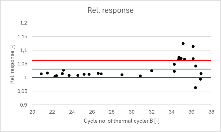
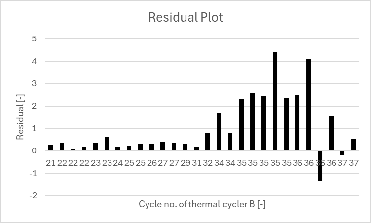
Evaluating the data using the relative response, we can see, that the values are outside the (self-selected!) limits starting from a Ct value of 34.73, while an examination of the residual plot already reveals a clear abnormality beginning with the Ct value of 32. This indicates that the linear model is no longer suitable for this part of the data.

In summary, it can be stated that the upper limit of linearity can be objectively determined using the statistical methods "relative response" and "residual analysis". Which method is ultimately to be used with which details is either specified in internal guidelines or should be decided by the user with appropriate justification.

 

¹ We can therefore safely ignore everything about the linear range of usually 80-120% (or 70-130% for content uniformity), as it is not relevant here.