About small values with huge influence - Sum Of Squares - part 2
In the first part of this blog article we became familiar with the RSS and started to get an insight about the influence of the individual data values. This is followed by this part.
Hat Values and Cook’s Distance – what is really influencing the regression line?
So far, we were thinking about the influence of data points, but have actually not clarified what influence actually means. One intuitive way to think about that is to consider what would happen to the regression line if a single data point would be removed from the data set. If one data point has a big influence on the regression line, then, removing that data point should change the regression line a lot, which can be measured by a difference in the slope and/or y-intercept. This can be done and is shown in the following Figure 1:
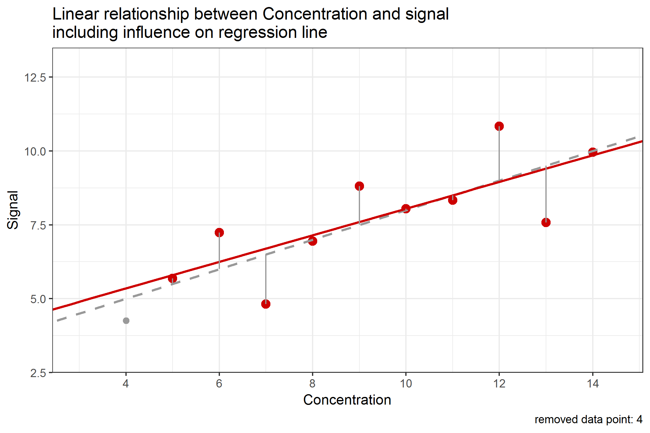
Figure 1: Change of the regression line by removing single data points when calculating
We have noticed (from Table 4, see last blog article) that the data point with concentration 9 has about 12% contribution to the RSS. But leaving this data point out of the data set would merely change the slope or intercept of the regression line. In contrast to that, leaving out data point with concentration 4 would influence the regression line in a similar manner, although this data point only has a 4% contribution to the RSS. This is an example showing that a data point being “far away” from all other data points has a higher influence to the regression line than data points being close to the center of the data set. This type of influence is called leverage and data points with high leverage are called high-leverage points. In method validation, it is important to notice that high-leverage points are most likely data points with very low (or high) concentrations, e.g. those close to the limit of quantification or detection (LOQ / LOD). But especially these values must be very "accurate" (let's better say "true"). Because of that, we have to carefully investigate the influence of these data points on the regression line.
Depending of the number of data points n, there is a limit for which a data point will likely be a high-leverage data point. In our example, this limit will be 2 * (2/n) = 0.363, where n = 11. A synonym for leverage is Hat Value or H Value. A visual representation is given in the following Figure 2, indicating that in our example, there are no high-leverage points. The data points for the concentrations 4, 5, 13 and 14 are possessing high leverage values as they are “far away” from the other data points. But as their leverage values are below the calculated limit of 0.363, they aren’t high-leverage points.
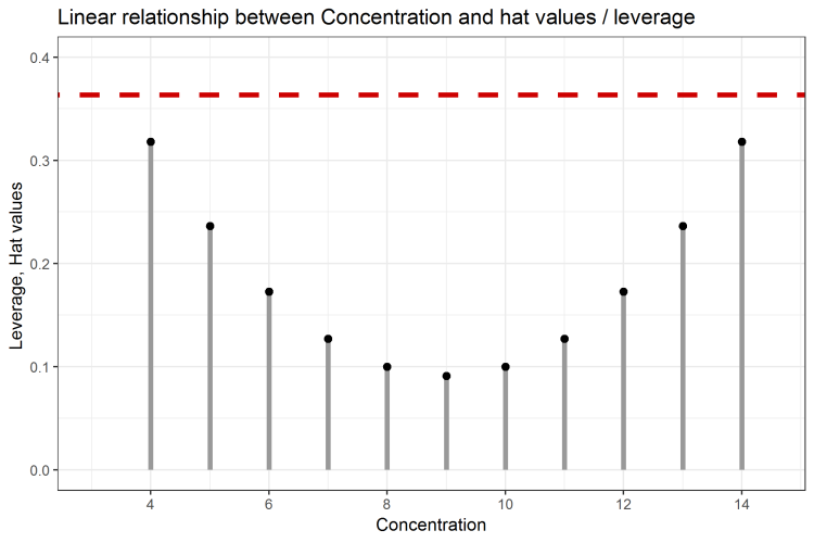
Figure 2: Leverage of each data point, and relation to hat value limit of 0.363
It is also important to clarify that data points with higher leverage don’t imply that they have a big influence on the regression line because they are only dependent on the X-coordinate (or analyte concentration in this case). Y values (or signal values in our case) are of no importance for the calculation of the leverage. Thus it is possible that data points with low leverage values do possess a high influence on the regression line and hence the quality of the method. Therefore, to fully investigate the influence of a data point, we need to have an additional measure that also takes the Y values into account.
A measure that takes the X and Y coordinate for each data point into account is the so-called Cook’s Distance (D) [1]. It relates each data point to all other data points, depending on the X and Y coordinates and is therefore giving a better measure for identifying so-called influential observations. These D values should be as small as possible and less than a limit which, for D, is calculated as 4/(n-2), with n representing the number of data points. In Figure 3, all data points are represented as Cook’s Distance and the limit here is 4 / 9 = 0.445. Consequently, data point x = 13 is identified as an influential observation, meaning, it would change the slope and / or y-intercept too much when removed. But, when looking only at its leverage this data point would not be identified as unusual.

Figure 3: Cook’s Distance used to identify influential observations
The values of Cook’s Distance are a mixture of the RSS and the leverage values. They combine the characteristics of all single data points by investigating the Y and X coordinates in relation to all other data points. Only with this combined measure the actual influence of a single data point can be revealed. To include this knowledge into the standard scatter plot and regression line, one might color-code data points having a statistical influence onto the whole data set. A figure containing all information might look like Figure 4. Here, the data, the regression line, and the information about the influence of each data point, is shown. The threshold is 0.445 and it can be seen that data point 13 is indicated an influential data point (blue color). Also, it should to be remembered, that this information couldn’t be made visible by only focusing on the residual sum of squares. Even for a “low” RSS value, there still might be influential data points present in the data set.
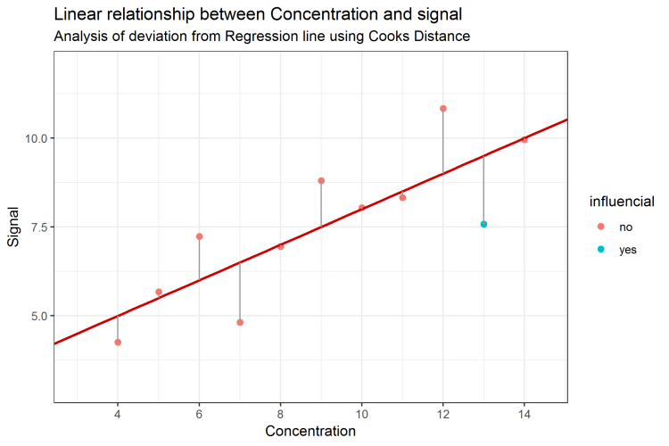
Figure 4: Linear regression and influential data point identified by Cook’s Distance
So, what to do when investigating linearity?
The ICH Q2(R2) requirement of „analysis of the deviation of the actual data points from the regression line” can easily be assessed using programs like Excel or other software solutions. When it comes to presenting the residual sum of squares, one needs to be sure what the RSS means. Good scientific interpretation can only be possible when investigating each data point because each data point has its unique contribution to the overall RSS. Visual inspection of the data is required, but cannot provide scientific justification, therefore one should always perform further “residual” analysis – not only to satisfy ICH Q2(R2) requirements, but also to gain knowledge about its own data.
The regression line, defined by slope and y-intercept reflects the general physico-chemical relation between concentration and signal. This relationship, based on the data, can be inaccurate and lead to wrong decisions, if influential data points are present and ignored. In that case, one should always check, why the influential data points behave differently than all the others. Also, influential data points are not necessarily outliers. Oftentimes, they reflect the natural behavior and higher variability in certain concentration ranges.
Conclusion
The residual sum of squares is a statistic value which is applied e.g. in linear regression. Its importance is often neglected, but when falsely interpreted it can lead to misunderstandings. In the same way that the average summarizes the properties of many data points in one value, the information about the individual values is lost. Regarding RSS, the individual contributions of the error squares are lost. Therefore, they must be separately analyzed to interpret the RSS correctly. Statistical key figures such as hat values / leverage or Cook’s Distance are useful to classify the contributions of the individual values correctly and thus help in the proper interpretation of the residual sum of squares.
In analytical method validation, general linear regression key performance indicators must be specified while an indication of the RSS is not required anymore. The performance of the residual analysis is mandatory. In obvious cases, a visual analysis of the residuals may be sufficient, but it is unable to identify potential influential data points. However, it is precisely these influential observations that may jeopardize the fitness-for-purpose of the method’s linearity, as they might distort the established linear relationship between analyte concentration and signal. Visual analyzes are always subjective - "scientific justification", on the other hand, can only be obtained by objective criteria, such as Cook’s Distance or similar methods for residual analysis.
When evaluating (e.g. linear) regression methods, the residual sum of squares constitutes the starting point of an interesting journey, ending in the knowledge about what the (linear) relationship is actually worth.
RSS, leverage and Cook’s Distance in Excel 2016
Prerequisites
It is possible to calculate the discussed measures in Excel 2016: The example discussed above is taken from a publication of Francis Anscombe [2]. The publication contains four data sets, the well-known Anscombe Quartet. These data sets are identical in many linear regression characteristics, although consisting of completely different data points. Here, we work with the first of these data sets (Table 1).
Table 1: Data set used in the example
| Data point | X value |
Y value |
| 1 | 4 | 4.26 |
| 2 | 5 | 5.68 |
| 3 | 6 | 7.24 |
| 4 | 7 | 4.82 |
| 5 | 8 | 6.95 |
| 6 | 9 | 8.81 |
| 7 | 10 | 8.04 |
| 8 | 11 | 8.33 |
| 9 | 12 | 10.84 |
| 10 | 13 | 7.58 |
| 11 | 14 | 9.96 |
When transferring these data into Excel, we here assume that the X values (e.g. analyte concentration) and the Y values (signal) will be stored in columns A and B. For analysis, first, we click onto “Data” and “Data Analysis”. There will be a new window from which we select “Regression”. Then, we enter the X and Y values cell ranges from the Excel sheet, e.g. columns A and B. It is important to activate the Residuals button, then we confirm by clicking “OK”. A new sheet is opening, where we will find all the information that we need for further analysis. These are stored in the following cells (Table 2):
Table 2: Characteristics in Excel for linear regression analysis
| Cell | Value | Formula / Symbol | |
| Multiple Correlation coefficient | B4 | 0.816 | r |
| Coefficient of Determination |
B5 | 0.666 | R2 (R2 = r * r) |
| Number of data points | B8 | 11 | n |
| RSS (residual sum of squares) | B14 | 13.762 | RSS = ∑ εi2 = (yi - ŷi )2 |
| y-intercept | B17 | 3.000 | Y value for X = 0, β0 |
| Slope | B18 | 0.500 | β1 |
| Estimates for Y | B25:B35 | ŷ | |
| Residuals | C25:C35 | ε = y - ŷ |
Since we will need the raw data and the values for the residuals for future calculations, we will merge them into one sheet. I merged the raw data into the new sheet, resulting in having the data point number in column A, the Y estimates in column B, the residuals in column C, and then analyte concentration and signal in columns D and E, they are shown from row 25 to 35 (Figure 5):
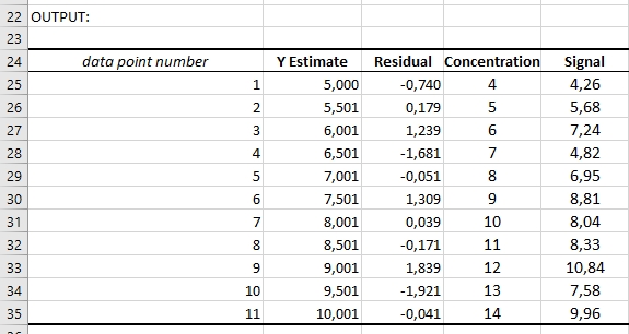
Figure 5: Data preparation: data for linear regression and residual analysis
To calculate the values for Cook’s Distance D for all data points i, Di, we need the formula: Di = (isri2) / p * hi /(1-hi). In order to do so, we need to calculate two more things, namely the leverage hi and squares of the isr values. These can be calculated from the residuals, which we already have.
Calculation of Residual Sum of Squares
The residuals for each data point can be calculated in the sheet be subtracting the Y estimates from the signal values, or E25 - B25 (for the first data point). The RSS then is the sum of all the squared residuals (E25 – B25)^2. Here, I put the residuals into column F (cells F25:F35) and the squared residuals into column G (cells G25:G35), see Figure 6. The value of the sum, or RSS, I will save in cell F37, its value will be the same as in cell B14, which is part of the data analysis output.
Calculation of leverage or H values
For further calculations, we need the average values (the mean; x), as well as the standard deviation (sx) of all x values (concentration). The average of x we will get using AVERAGE(D25:D35), and we save it in cell D37. The standard deviation of x we will get using STDEV.S(D25:D35) and we save it in cell D38. We will need those for the following steps, the calculation of leverage respectively hat values: The formula for hat value calculation is hi = 1/n + 1/(n-1) * ((xi - x)/sx)2. Using the currently calculated values for x and sx, we use the following Excel formula to calculate the hat value for the first data point (D25): (1/$B$8) + 1/($B$8-1) * (($D25 - $D$37) / $D$38)^2. Again, as stated above, we recognize that leverage is just depending on the x values (concentration, column D) of the data and on its relation to the other values (indicated with cells D37 and D38), but not on the y values (signal).
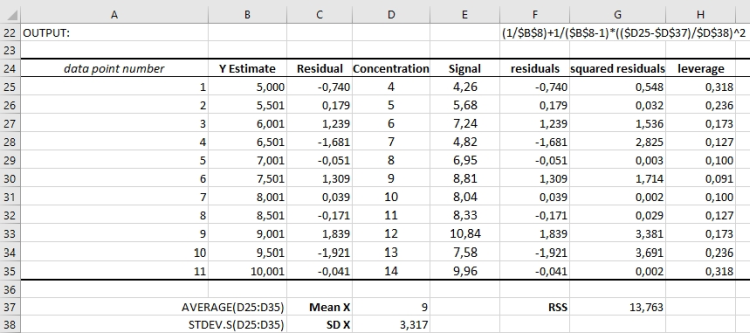
Figure 6: Calculation of leverage
Calculation of Cook’s Distance / D values
Now, we use the leverage to calculate the Cook’s Distance. For that, we first calculate the isr value for each data point: isri = εi / (sE √(1 - hi)). εi are the residuals, which we already have calculated in column C and F. We saved the leverage values hi in column H. Value sE can be calculated with SQRT(($B$8-1)/($B$8-2)*STDEV.S(F25:F35)^2), we save it in cell D39. Therefore, the isr for the first data point (row 25) is: F25/$D$39/SQRT(1-$H25), we save all isr values in column I.
With that, we calculate Cook’s Distance D. For data point i, we calculate Di as follows: Di = (isri2) / p * hi /(1-hi) and for data point 1 (row 25), we have: $I25^2 / 2 * $H25 / (1-$H25). We save all values in column J. That is everything we need to calculate the Cook’s Distance in Excel, thus being able to provide all information; not only regression analysis but also residual analysis.
The following Figure 7 shows a summary of all the steps taken:
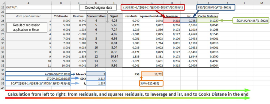
Figure 7: Overview over all steps needed to calculate leverage and Cook’s Distance for a given data set based on linear regression in Excel 2016.
Sources
[1] Cook’s Distance: Cook, R. Dennis (February 1977). "Detection of Influential Observations in Linear Regression". Technometrics. American Statistical Association. 19 (1): 15–18.
[2] Anscombes Quartett: F. J. Anscombe: Graphs in Statistical Analysis. In: American Statistician. 27, No. 1, 1973, page 17–21.
Did you like this article? Then, you've got the possibility to download the whole article as pdf by clicking here.
About the author
|
|
Dr. Peter P. Heym wrote this article as guest author. He studied bioinformatics and obtained his PhD at the Leibnitz Institute for Plant Biochemistry Halle with the topic "In silico characterisation of AtPARP1 and virtual screening for AtPARP inhibitors to increase resistance to abiotic stress". He is the CEO of Sum Of Squares - Statistical Consulting (www.sumofsquares.de), a service company specialized in statistical consulting for students, individuals, and companies. In addition to statistical advice he offers support for university thesis, evaluation of surveys, workshops (e.g. in programming language R), seminars, and trainings, also in GMP topics. |