Linearity tests
Many analytical methods require calibration to determine the linear range. Linearity tests can be used to check whether the determined calibration function is actually linear.
Depending on the scope / “business area”, checking the linearity using linearity tests is also required for method validations or could at least be useful. In an earlier article, we looked at the relative response in this context.
In the meantime, however, I came across other linearity tests and we will have a look at these in today's article.
Linearity test: "Point-to-point slope"
The linearity test checking the "point-to-point slope" reminded me a bit of the calculation method for the relative response. It is described, for example, in the current DIN 38402-51 (from 2017), where it replaces the linearity test according to Mandel recommended by older standards. It requires at least 6 concentrations distributed equidistantly, and the slopes are calculated from the data of 2 consecutive measuring points. Then - in contrast to the calculation done for the relative response - the median is calculated (instead of the mean) and the individual values are compared with the tolerance limits applied to the median. A quality control chart presents the results.
An example of a photometric determination of nitrite looks like this (the example is taken from DIN 38402-51), and a 10% tolerance has been applied:
| No. of calibration standard | Concentration (xi) [µg/L] | Extinction (yi) [-] | Point-to-point slope (Δy/Δx) [1/µg*L-1] | Deviation from the median [1/µg*L-1] |
| 1 | 0.66 | 0.0037 | 0.00712 | -0.00023 |
| 2 | 1.32 | 0.0084 | 0.00735 | 0.00000 |
| 3 | 2.64 | 0.0181 | 0.00702 | -0.00033 |
| 4 | 5.26 | 0.0365 | 0.00712 | -0.00023 |
| 5 | 6.58 | 0.0459 | 0.00720 | -0.00015 |
| 6 | 7.90 | 0.0554 | 0.00733 | -0.00002 |
| 7 | 10.60 | 0.0752 | 0.00736 | 0.00001 |
| 8 | 26.00 | 0.1885 | 0.00777 | 0.00042 |
| 9 | 44.71 | 0.3339 | 0.00836 | 0.00101 |
| 10 | 63.19 | 0.4884 | 0.00901 | 0.00166 |
| 11 | 82.18 | 0.6595 | 0.01003 | 0.00269 |
| 12 | 100.00 | 0.8383 | - | - |
| Median | 0.00735 | - | ||
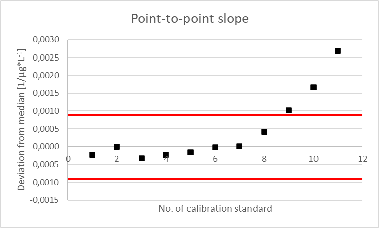
Taking into account the 10% tolerance, the statement is that linearity ends after the 8th calibration standard, i.e. the calibration range is limited to 0.66 - 26.00 µg/L.
Empirical curvature test
In addition to the linearity test examining the "point-to-point slope" just explained, DIN 38402-51 also deals with the empirical curvature test. In this test, the slope is determined for each measuring point in relation to zero. The test examines from which measuring point the regression line starts forming a curve. The 2nd degree polynomial (𝑦 = 𝑐𝑥2 + 𝑏𝑥 + 𝑎) is determined for the calibration data and the coefficient b is calculated from this function. Then you apply your internally defined tolerances (e.g. 10%) and calculate the threshold value R0. The algebraic sign of the quadratic part of the function must also be considered, as it provides information about the shape of the curve. If it is negative, it is a concave calibration curve and R0 would be 0.90 x b; for convex curves it is 1.10 x b. Then, the responsivity R = y/x is calculated for each individual measuring point (this is the same as the relative response) and compared with the threshold value R0. For convex calibration curves, R should be ≤ than R0, otherwise this measurement point belongs to the curved part.
Let's take another look at the example of the photometric nitrite determination. This example can be represented by the linear equation 𝑦 = 0.0082𝑥 - 0.0107, and the 2nd degree polynomial is 𝑦 = 0.00002𝑥2 + 0.0067𝑥 + 0.0008 (please refer to basic mathematical knowledge for the derivation of the quadratic equation). The quadratic part has a positive algebraic sign; thus, it is a convex curve and b is 0.0067. Multiplying by 1.1 (because 10%) results in a threshold value R0 of 0.00736:
| No. of calibration standard | Concentration (xi) [µg/L] | Extinction (yi) [-] | Responsivity R = y/z [1/µg*L-1] | Cf. with R0 (=0.00736) |
| 1 | 0.66 | 0.0037 | 0.00561 | R < R0 |
| 2 | 1.32 | 0.0084 | 0.00636 | R < R0 |
| 3 | 2.64 | 0.0181 | 0.00686 | R < R0 |
| 4 | 5.26 | 0.0365 | 0.00694 | R < R0 |
| 5 | 6.58 | 0.0459 | 0.00698 | R < R0 |
| 6 | 7.90 | 0.0554 | 0.00701 | R < R0 |
| 7 | 10.60 | 0.0752 | 0.00709 | R < R0 |
| 8 | 26.00 | 0.1885 | 0.00725 | R < R0 |
| 9 | 44.71 | 0.3339 | 0.00747 | R > R0 |
| 10 | 63.19 | 0.4884 | 0.00773 | R > R0 |
| 11 | 82.18 | 0.6595 | 0.00803 | R > R0 |
| 12 | 100.00 | 0.8383 | 0.00838 | R > R0 |
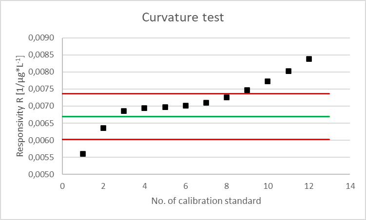
Analogous to the linearity test examining the "point-to-point slope", we also get the same statement applying this linearity test 😉.
If you are now wondering what is going on with the first calibration standard, as it is also outside the tolerance, the standard explains this by the offset and states that for calibration activities, we are only interested in curved part at the right side (responsivity for high concentrations).
Linearity test according to Mandel
Finally, a few words on Mandel’s (fitting) test. If the working range only extends over one decade, variance homogeneity is present (as previously required) and the measuring points are equidistantly distributed, Mandel’s linearity test provides good information as to whether the linear calibration function is sufficiently suitable compared to the quadratic calibration function. However, if the calibration line extends over several decades and the measuring points are distributed approximately equidistantly on a logarithmic scale, Mandel’s test very often results in a "non-linear" outcome, and the working range must therefore be restricted. For this reason, the 2017th version of DIN 38402-51 recommends the linearity test examining the point-to-point slope.
Nevertheless, the Mandel test will also be briefly presented here. For this test, the linear calibration function is compared with the 2nd degree calibration function. To do this, the residual standard deviations of both functions are calculated (how this works for a linear function is described here in the update of Nov. 3rd, 2023: check "SDresiduals"; now abbreviated as sy in this article). Afterwards, the residual variances (sy lin2 or sy quad2) are formed and the variance difference DS2 is calculated according to DS2 = (n-2) * sy lin2 - (n-3) * sy quad2. The test statistic TS is calculated according to TS = DS2 / sy quad2. As an F-test, TS is then compared with the F value of an F-table applying a significance level α = 0.01 and f1 = 1 and f2 = n-3. If TS is smaller than the tabulated F value, the difference between DS2 and the residual variance sy quad2 is not significant, and the calibration function can be regarded as linear in the investigated working range.
Without considering that in our example of the photometric nitrite determination, the working range covers slightly more than 2 decades, Mandel’s test will also be presented using this example:
| Linear function |
Quadratic function | |
| Functional equation | 𝑦 = 0.0082𝑥 - 0.0107 | 𝑦 = 0.00002𝑥2 + 0.0067𝑥 + 0.0008 |
| Residual standard deviation sy | 0.0146 | 0.0019 |
| Residual variance (sy lin2 or sy quad2) | 0.0002125 | 0.0000037 |
| Variance difference DS2 | 0.00209 | |
| Test statistic TS | 571.8 | |
| Tabulated F value | 10.56 | |
TS is significantly greater than the tabulated F value, so our example is of course not linear, which we already knew from the previous linearity tests. However, even if we limit the working range to up to 26 µg/L, TS is still greater than the corresponding F value. Only if the working range is narrowed down to 0.66 - 10.6 µg/L, we obtain the statement that this working range is linear...
To summarize, the linearity test examining the "point-to-point slope" seems to me to be the simplest from a mathematical point of view, as I don't have to determine the 2nd degree calibration function and other variables. We’ve already touched on the disadvantages of Mandel’s linearity test above. However, which test is best used when depends on the width of the working range, the distribution of the measuring points, personal preference, or internal specifications.