Inferring trueness from linearity – 1. Approach: Normalization
In today's blog, we’d like to address a quite common problem during method validations and by using a practical example showing possibilities to solve it.
A SE-HPLC method used as a purity test of a drug shall be validated. It's known that impurities (e.g. aggregates and / or fragments of the product) may arise in low concentrations. In the chromatogram, you’ll see the main peak corresponding to the intact product and a few minor peaks corresponding to impurities, which will be reported as sum.
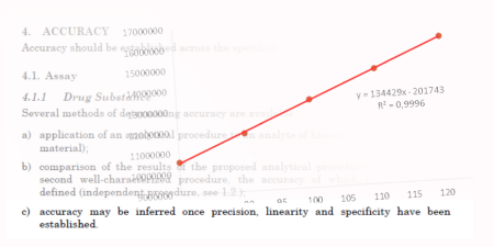
Let's have a look at the validation parameter trueness ("accuracy"). Unfortunately, neither impurities are separately available for spiking experiments nor independent alternative methods are existing. In this case, the validation guideline ICH Q2(R1) offers the following possibility for the evaluation of trueness: "Accuracy may be inferred once precision, linearity and specificity have been established" (4.1.1 c / 4.1.2 c).
That sounds interesting. Assuming the proof of specificity being no problem, we should be able to infer trueness from the linearity data and check if the results are also precise. This might be quite feasible.
So, let’s have a look at this using a concrete example. For the determination of linearity 5 concentrations were used (examination levels: 80%, 90%, 100%, 110%, 120% of the test concentration; for the sake of simplicity the real concentrations are omitted). Since these experiments were planned to additionally cover trueness, we have prepared 3 independent dilutions for each of these concentrations. After performing the experiments, we obtained the following data set regarding absolute peak areas:
| Absolute peak area [µAU*s] | ||
| Examination level (%) | Sum of minor peaks | Main peak |
| 120 | 99104 | 15949990 |
| 96153 | 15988085 | |
| 97723 | 15879248 | |
| 110 | 89383 | 14567078 |
| 87474 | 14592610 | |
| 88355 | 14558575 | |
| 100 | 77587 | 13275901 |
| 76162 | 13264078 | |
| 78209 | 13285496 | |
| 90 | 65802 | 11513839 |
| 67811 | 11937356 | |
| 68012 | 12037029 | |
| 80 | 54208 | 10489899 |
| 55611 | 10594228 | |
| 56819 | 10683872 | |
For the determination of linearity, the peak areas were plotted against the real concentrations for both the sum of minor peaks and the main peak, and regression lines each having a coefficient of determination of R2 > 0.99 were obtained (not shown here). Thus, the predefined acceptance criterion for linearity is met and linearity is clearly proven. Hence, we are allowed to use these data for the evaluation of trueness.
Before we turn to the evaluation of this data set, we should recap what we want to show. Trueness is defined as follows: „The accuracy of an analytical procedure expresses the closeness of agreement between the value which is accepted either as a conventional true value or an accepted reference value and the value found.“. This means that we’d like to examine how well a measured value corresponds to the real theoretical value. We’ve got the measured values, but how can we determine the theoretical values? For this, different approaches exist - today we’ll perform it applying normalization and in a future blog article, we will show another way.
Hm, so how to normalize?
Applying normalization, we will be able to compare all obtained values with the 100% examination level value. For this purpose, each measured value is multiplied by 100 and then divided by its examination level (for example, first minor peak value: 100 * 99104 / 120 = 82587). Thus, we convert them all to 100% and our data set looks like this:
| Absolute peak area [µAU*s] | |||
| Examination level (%) | Normalized level (%) | Sum of minor peaks | Main peak |
| (120) | 100 | 82587 | 13291658 |
| 80127 | 13323404 | ||
| 81436 | 13232706 | ||
| (110) | 81257 | 13242798 | |
| 79521 | 13266009 | ||
| 80322 | 13235068 | ||
| (100) | 77587 | 13275901 | |
| 76162 | 13264078 | ||
| 78209 | 13285496 | ||
| (90) | 73114 | 12793154 | |
| 75345 | 13263729 | ||
| 75569 | 13374477 | ||
| (80) | 67759 | 13112373 | |
| 69513 | 13242785 | ||
| 71024 | 13354840 | ||
When looking at the numbers, we observe that at least the numbers of the main peak are all quite similar and that the ones of the minor peaks do not differ so much. But what is “do not differ so much”? Mathematically, this can be expressed by the relative standard deviation (RSD). We first calculate the mean and standard deviation (SD) and then divide the standard deviation by the mean and multiply by 100, which gives us the result in percent.
In our example, we obtain the following data:
| Sum of minor peaks | Main peak | |
| Meanabsolute peak area [µAU*s] | 76635 | 13237232 |
| SDabsolute peak area [µAU*s] | 4581 | 136803 |
| RSD [%] | 6.0 | 1.0 |
As we already can see when examining the numbers, the RSD of the main peak with 1% and that of the minor peaks with 6% is either very good or in the ballpark. So what does this mean, when we look back at the definition of trueness? It shows that our measured values, when we convert them to 100%, correspond very well to the theoretical one, and thus our measurement is really very true. So, we can use the relative standard deviation of normalized values as an acceptance criterion for the determination of trueness based on linearity data. Telling general limits to be used as acceptance criteria is not possible. They are based on the permissible error and the maximum possible trueness of the method. In our example, however, we would be fine with an acceptance criterion of RSD ≤ 10% for the sum of minor peaks and of RSD ≤ 2% for the main peak ;-)
There was something else... - what about precision?
Yes, right, the ICH Q2(R1) additionally stated that precision should also be considered: "Accuracy may be inferred once precision, linearity and specificity have been established".
So, using once more our data set, we now take a look at the relative peak areas (in area%) instead of the absolute ones. Usually, they are already evaluated by chromatography system’s software. Alternatively, of course, we could also calculate them on our own, by calculating for each peak its percentage in relation to the sum of all peaks. In our example it looks like this:
| Relative peak area [area%] | ||
| Examination level (%) | Sum of minor peaks | Main peak |
| 120 | 0.6175 | 99.3825 |
| 0.5978 | 99.4022 | |
| 0.6116 | 99.3884 | |
| 110 | 0.6099 | 99.3901 |
| 0.5959 | 99.4041 | |
| 0.6032 | 99.3968 | |
| 100 | 0.5810 | 99.4190 |
| 0.5709 | 99.4291 | |
| 0.5852 | 99.4148 | |
| 90 | 0.5683 | 99.4317 |
| 0.5648 | 99.4352 | |
| 0.5618 | 99.4382 | |
| 80 | 0.5141 | 99.4859 |
| 0.5222 | 99.4778 | |
| 0.5290 | 99.4710 | |
Theoretically, we expect that when setting peak areas in relation to each other, they should always be the same regardless of the dilution and are thus only influenced by precision. Therefore, we again determine the relative standard deviation:
| Sum of minor peaks | Main peak | |
| Meanrelative peak area [area%] | 0.5756 | 99.4244 |
| SDrelative peak area [area%] | 0.0330 | 0.0330 |
| RSD [%] | 5.73 | 0.03 |
We realize that the thesis above is quite true for the main peak, however, for the sum of minor peaks a dilution effect is seen (at 120%, the mean is about 0.61 area%, at 100% it’s 0.58 area% and at 80% it’s only 0.52 area%). Accordingly, the precision at these very low amounts is not as fantastic as the one of the predominant main peak. Depending on which acceptance criteria were chosen, however, this can still be completely maintainable.
In summary, we can note that we can infer trueness from linearity data (absolute peak areas) by normalizing to 100% and considering the relative deviation thereof and by evaluating precision using relative peak areas, when specificity is given (as we have just assumed here).