How to determine the LOD using the calibration curve?
In case of purity tests during method validation, it is necessary to determine the limit of detection (LOD, sometimes also called DL = detection limit) and the limit of quantification (LOQ), respectively. This can be done e.g. based on the calibration curve and is then called “calibration curve procedure” in the (German) literature.
Using the detection limit as example, the validation guideline ICH Q2(R1) specifies the following requirements in section 6.3 and 6.3.2:
The calculation is as follows: DL = 3.3x σ / S where S is the slope of the calibration curve and σ is the standard deviation of the response. And exactly this standard deviation can be determined in different ways, i.a. by the use of the calibration curve:
„A specific calibration curve should be studied using samples containing an analyte in the range of DL. The residual standard deviation of a regression line or the standard deviation of y-intercepts of regression lines may be used as the standard deviation.“.
That sounds interesting. Since we were not confronted with this topic in any customer project yet, I wanted to find out how to do this in practice. That shouldn’t be so hard, I thought. But I learned quickly that I was wrong as different opinions exist. During research, I saw quite a lot of different possibilities.
Just one or many calibration curves – and what’s the background?
All agree to and given by the guideline is the fact that the "normal" calibration curve spanning the working range (as determined in the linearity experiments) shouldn’t be taken. Instead, one calibration line covering the lower range in the presumed environment of the detection limit should be applied. This has a simple mathematical background: when using the "normal" calibration line, which has considerably higher values, the center is shifted to a higher value, too. Thus, any detection limit derived from this line would also possess a much too high value. Therefore, it is recommended to use not more than 10 times of the presumed detection limit as highest concentration for the LOD determination calibration curve [1, 2].
Ok, so let’s use a calibration line in the area of the LOD. Alright, but should it be just one? And with how many concentrations?
Concerning this matter, the most diverse opinions exist. Mathematically, it would be possible with just one line; but also two or more lines or multiple injections are used. Before we take a look at these possibilities in practical examples, we should first of all deal with the mathematical background.
A regression line (y = mx + c) is based on the method of the least squares. Since not all data points are 100% on the line, the line maps the best possible adjustment. Accordingly, there is an inherent standard deviation. Visualized it looks like this:
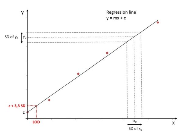
In this figure, please consider that the widths for the standard deviations are strongly enlarged and therefore the way LOD is presented here, doesn’t really correspond to 3.3*SD...
Considering 3.3 times the standard deviation, we can calculate the Y-intercept of the LOD using the formula: yLOD = 3.3 σ + c and the LOD concentration (x) as x = (yLOD-c) / m. Combined, this results in x = 3.3 σ / m, which is the formula given above by the ICH.
Mathematically, the following conditions apply when using the calibration curve procedure [2]:
- there is linearity in the area of the presumed LOD (otherwise this whole approach doesn’t make any sense)
- the response values of the samples are normally distributed and independent of each other
- there is variance homogeneity in the calibration area.
Since in practice these conditions are not necessarily 100% met, it must be kept in mind that the determined value can be based on a certain degree of inaccuracy.
A practical example for illustration
Let's take a closer look using a practical example. Based on values of real experiments, values for 4 lines with 5 measurement points each with 3 replicates in the area of the suspected LOD were constructed. In the real experiment, a LOQ of the RP-HPLC method previously determined during method development was verified applying the signal-to-noise method. The LOQ was determined to be 6 μg/mL. Thus, the suspected LOD was derived being 1.8 μg/mL.
The following table shows the mean values of the "measurement values" of these constructed experiments:
| Experiment 1 | Experiment 2 | Experiment 3 | Experiment 4 | |
| Conc. [µg/mL] | Area [µAU*s] | |||
| 1.8 | 25364 | 25776 | 27016 | 25566 |
| 4.2 | 68407 | 68527 | 69041 | 68568 |
| 6.6 | 108226 | 108239 | 109760 | 108342 |
| 10.8 | 173944 | 173497 | 175987 | 173747 |
| 15.0 | 235865 | 235474 | 247231 | 235686 |
These measurement values were subjected to regression analysis and the regression line with slope m, Y-intercept c, coefficient of determination R2 and the residual standard deviation and the standard deviation of the Y-intercept were determined. There are several options for this in Excel. One is the application of the LINEST function, which can be perceived as somehow tricky. Another one is the way using the tab "Data" → "Data analysis" → Regression → select the data to be examined and click on the field "Residuals" → click on "ok", and an output window with a multitude of statistically interesting information will open. Among these are, of course, also the information about the residual standard deviation (in field B7) and that of the Y-intercept (in field C17). VERY IMPORTANT: Even though these fields are displayed as SE (= standard error) by Excel, they are really SD and NOT SE. I have checked this, see section below. For a detailed explanation of these functions, the reader might be recommended to watch YouTube videos ;-)
The following results were obtained:
| Experiment 1 | Experiment 2 | Experiment 3 | Experiment 4 | |
| Regression line | y=15878x+416 | y=15814x+849 | y=16562x-1389 | y=15844x+699 |
| R2 | 0.9987 | 0.9988 | 0.9997 | 0.9987 |
| Slope m | 15878 | 15814 | 16562 | 15844 |
| Y-intercept c | 416 | 849 | -1389 | 699 |
| SDY-intercept | 2943 | 2849 | 1429 | 2937 |
| SDResiduals | 3443 | 3333 | 1672 | 3436 |
[Small remark: Interestingly, the values calculated for the coefficient of determination R2 may differ from those shown in figures... but is another story.]
With the values obtained for the standard deviation of the Y-intercept or the residual standard deviation, the LOD can now be calculated in accordance with the known formula LOD = 3.3 SD / m:
| Experiment 1 | Experiment 2 | Experiment 3 | Experiment 4 | |
| LOD in µg/mL calculated using SDY-intercept | 0.61 | 0.59 | 0.28 | 0.61 |
| LOD in µg/mL calculated using SDResiduals | 0.72 | 0.70 | 0.33 | 0.72 |
In this constructed example, the results don’t differ very much apart from experiment 3. For reality, it is certainly advisable to evaluate more than just one line (whether it must be 4 is another question) and at best, to generate independent results, to perform the experiments on different days and by different testers. To what extent this effort is justified remains up to you.
When looking at the results, it is also interesting to note that with a mean value of 0.66 μg/mL (excluding experiment 3) they are a bit lower than the initially assumed LOD of 1.8 μg/mL. However, this may already be due to the fact that another evaluation technique was used to determine the LOQ (see also next section).
The number of lines and measurement points used in the example does not claim that LOD determinations must be performed in exactly this way. On the contrary, it should act as a starting point for discussion, as also other possibilities were seen when doing research for this blog article. Thus, e.g. 2 lines (one above and one below the presumed LOD) might be another interesting option, and a different calculation is used in the guidance document for the LOD and LOQ determination of contaminants in feed and food [2]. Of course, such a document is of no regulatory relevance for drugs but may possibly also be an option for orientation.
Different evaluation techniques result in different results
A quick look at two publications [3, 4] shows that the results differ depending on which method is used to determine the LOD and LOQ (visual examination, signal-to-noise, or the calibration line method described in this blog post). Even within the calibration line method quite different results can be obtained, depending on whether the residual standard deviation or that of the Y-intercept is used.
From a regulatory point of view, no justification for the method of determination used is necessary. From the scientific point of view, this is questionable to me.
What are your experiences and what is your point of view?
Update 03.11.2023: Use of SD or SE?
For this article I received questions from time to time, about what should be used for the calculation of the LOD by means of calibration line method: SE or SD? There is some confusion about this, which may be due to the incorrect designation of SE for SD in Excel, as already mentioned above. Accordingly, there are also many discussions on the topic of SE vs. SD for LOD calculation.
However, very nice are the explanations of this topic in [5]. With the help of the explanations given there, I have verified exemplarily the way of calculation for the calibration line of experiment 1 shown above. For this purpose, I calculate some auxiliary values as shown in the following table:
| Conc. (xi) |
Response (yi) |
(xi-X̅) | (xi-X̅)2 |
ŷi |
(yi-ŷi) | (yi-ŷi)2 |
xi2 | ||
| 1.8 | 25364 | -5.9 | 34.6 | 28997 | -3633 | 13197214 | 3.2 | ||
| 4.2 | 68407 | -3.5 | 12.1 | 67105 | 1302 | 1695469 | 17.6 | ||
| 6.6 | 108226 | -1.1 | 1.2 | 105213 | 3013 | 9080934 | 43.6 | ||
| 10.8 | 173944 | 3.1 | 9.7 | 171902 | 2042 | 4170512 | 116.6 | ||
| 15 | 235865 | 7.3 | 53.6 | 238590 | -2725 | 7425333 | 225.0 | ||
| n = 5 | |||||||||
| Mean (X̅) | 7.7 | - | Sum | - | 111.2 | - | - | 35569461 | 406.1 |
The first two columns "Conc." and "Response" are taken from the very first table of this article. For the concentrations I calculate the mean value X̅. I subtract the mean from each individual value (xi-X̅). The values thus obtained are squared ((xi-X̅)2) and summed (∑(xi-X̅)2, here: 111.2). To be able to calculate ŷi (these are the theoretical values), I first have to calculate the slope of my regression line (15878) and its y-intercept (416). Then, by inserting the respective xi values into the regression line’s equation (y = 15878*x + 416), I can determine the corresponding theoretical ŷi values. By subtracting ŷi from yi, I can calculate the residuals (yi-ŷi), and then square them ((yi-ŷi)2). The sum of them is the RSS (residual sum of squares, here: 35569461). Further, we need the sum of the squared xi values (∑xi2, here: 406.1).
Using the following formulas, I can finally calculate SDResiduals and SDY-intercept:
SDResiduals = √(RSS/(n-2)) = √(35569461/3) = 3443
SDY-intercept = SDResiduals * √((∑xi2 / (n * ∑(xi-X̅)2))) = 3443 * √((406.1 / (5 * 111.2))) = 2943
And “surprisingly”, these are exactly the values that Excel incorrectly output as SEs in the regression analysis above....
By the way, in a very interesting discussion on SE versus SD for LOD calculation using calibration line at ResearchGate, I also came across the following: SD provides information about the statistical spread within a (small) sample (n), while SE refers to the variability within the population (N). Therefore, a corresponding suggestion, which is very obvious to me, was to use SD at the beginning / during method development, when only a small sample is available and the information base is not yet that accurate, and to use SE later, when the method is already fully developed, and a larger data set is available. Since SE is lower than SD, using SD to calculate LOD at the beginning of the project is a conservative approach since correspondingly higher values are obtained. Later, when the method will be used routine work, the use of SE (based on a larger data set) can then subsequently provide a better estimate for LOD.
Nevertheless, we should keep in mind that, in general, a LOD calculated in this way is basically only a rough estimate and should be verified experimentally using samples diluted close to the calculated concentration, as is required by ICH Q2(R1).
References
[1] Kromidas S. (2011). Validierung in der Analytik (validation in analytics), Wiley-VCH Verlag GmbH & Co KGaA, Weinheim, ISBN 978-3-527-32939-7
[2] Robouch P., Stroka J., Haedrich J., Schaechtele A., Wenzl T. (2016). Guidance document on the estimation of LOD and LOQ for measurements in the field of contaminants in feed and food
[3] Saadati N., Abdullah M.P., Zakaria Z., Sany S.B., Rezayi M., Hassonizadeh H. (2013). Limit of detection and limit of quantification development procedures for organochlorine pesticides analysis in water and sediment matrices, Chem Cent J., Vol. 7(1):63
[4] Şengül Ü. (2016). Comparing determination methods of detection and quantification limits for aflatoxin analysis in hazelnut. J Food Drug Anal., Vol. 24(1):56-62.
[5] Ellison S.R.L., Barwick V.J., Duguid Farrant T.J. (2009, 2nd edition). Practical Statistics for the Analytical Scientist: A Bench Guide, RSC Publishing, Cambridge, ISBN 978-0-85404-131-2
P.S.: This article for the detection limit LOD can of course also be transferred to the limit of quantification LOQ using the appropriate formula.