About small values with huge influence - Sum Of Squares - part 1

Often, the small things make the biggest difference in life. Sometimes these things we do not recognize at first as big but as soon as we draw our attention to them, they become more important.

In analytical method validation, one of these small things is the so-called sum of squares or residual sum of squares (RSS). The (residual) sum of squares you will often find as a number in validation reports that, at first sight, might be of no interest at all. That is why, in this article, we will explain in more detail what this number actually means and why it is of importance. We will discuss its meaning and its importance, as well as the pros and cons and what can be done to avoid statistical pitfalls when using the RSS.

 

Analytical Method Validation and ICH Q2(R1)

When validating an analytical method, the ICH guideline Q2(R1) is of importance. This guideline describes which characteristics of the method need to be evaluated in order to verify that a method is suitable for its intended purpose (fit-for-purpose). How to do that is well-described in detail in “Validation of Analytical Procedures: Text and Methodology Q2(R1)“, where ICH stands for International Council for Harmonisation of Technical Requirements for Pharmaceuticals for Human Use. For assays or quantitative impurities, not only characteristics as specificity and range, or trueness and precision have to be evaluated, but also, the linearity of the method needs to be assessed. Linearity in this context is defined as the ability (within a given range) to obtain test results which are directly proportional to the concentration (amount) of analyte. The basis for evaluating linearity is the linear relation between the analyte concentration and the signal. It is easy to visualize the data and the linear relationship, as displayed in Figure 1.

 

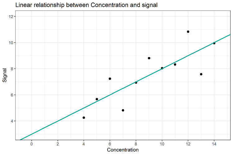
Figure 1: Linear Relationship between analyte concentration and signal

Using simple linear regression, the relation between analyte concentration and signal can be established. Here, with increasing concentration, a signal of increasing intensity is observed. The linear relationship can be described using the slope and the y-intercept of a straight line. In the example, at a concentration of 0, we would still get a signal intensity of 3. And for every increase in one concentration unit we would get an increase of 0.5 units of signal intensity. Therefore, the mathematical relationship between concentration and signal would be: signal = 3 + 0.5 * concentration or y = 3 + 0.5 * x. It is not difficult to use programs like Excel or other statistical tools to identify this relationship, when applying simple linear regression and the method of least squares. How to do this will be explained later (in part 2).

Considering the actual data points, we notice that, for example, we have actually observed a signal of 8.81 for a concentration of 9. Inserting concentration x = 9 into the equation would result in a concentration of 3 + (0.5 * 9) = 7.5. The measured values and regression line prediction do actually differ. The regression line describes the best-possible linear relationship between signal and concentration, and still, it is not capable of exactly predicting the observed values due to the fact that every single measurement value is deviating from the regression line. These differences of observed vs. predicted values are the reason why the regression line is not able to describe this relation 100% exactly. In our example, the regression line can only describe this relationship with 66.7%. This percentage corresponds to the well-known characteristic “coefficient of determination”, or R² and it describes the percentage of variability in the data that can be explained by the applied regression line. The remaining percentage of 33.3% remains unexplained by the regression line.  

 

Will one graph be enough to match ICH Q2(R1) requirements?

Let’s assume we already have calculated the regression line describing the linear relationship between concentration and signal, hence we also know its slope and y-intercept. Using Excel or other tools for calculating the regression line we also know the coefficient of determination. Are these measures enough to define our method as being fit-for-purpose regarding linearity? Let’s have a look into the guideline:

“A linear relationship should be evaluated across the range … of the analytical procedure. … Linearity should be evaluated by visual inspection of a plot of signals as a function of analyte concentration or content. If there is a linear relationship, test results should be evaluated by appropriate statistical methods, for example, by calculation of a regression line… . The correlation coefficient, y-intercept, slope of the regression line and residual sum of squares should be submitted.”

Most of the characteristics were already calculated. A graphical representation of the data and the regression line (including the formula showing slope and y-intercept) can be set up easily in Excel, the R² value can be included in the figure with a single click in Excel as well. Rooting R² results in r, which is the correlation coefficient, also required by the ICH Q2(R1). According to ICH Q2(R1), we already have almost everything we need to address for evaluating linearity. The only thing left is hidden in the last sentence. So, the last thing we need to clarify is the residual sum of squares.

 

From single values to residual sum of squares

What is the so-called residual sum of squares, which is oftentimes abbreviated with RSS? Is there any link from the data or regression line to the RSS? And why would we need this value to satisfy ICH Q2(R1) requirements? As we have already noticed, the regression line predicts a signal of 7.5 for the concentration of 9, although the actual measurement was 8.81. We keep in mind that the R²=0.67 means that the regression line is able to explain only 67% of variation in the data. Therefore, the remaining 33% of variation cannot be explained by the regression line. This corresponds to the fact, that the regression line predicts values for the signal which are different from the actual values. As in the example of concentration 9, the regression line predicts a signal of 7.5, which deviates by 1.31 units from the actual data point  (8.81 - 7.50) = y - ŷ = 1.31. In this case, the regression line underestimates the actual value by 1.31 units. Similarly, the difference between the predicted and actual signal for concentration 8 is (6.95 - 7.00) = -0.05, meaning that here, the regression line overestimates the signal by 0.05 units. This difference is called error, residuum or residual, and is often denoted by ε (epsilon). The residuum for concentration x = 4 we would write as follows: ε₁ = y₁ - ŷ₁ = 4.26 - 5.00 = -0.74. Graphically, we can illustrate the residuals of each data point as grey lines in the scatter plot (Figure 2). The length of each line corresponds to the magnitude of prediction error, ε, for each concentration. Why don’t we sum up all the errors to get one value for the total error of prediction? Wouldn’t this correspond to the “goodness” of the model?

 

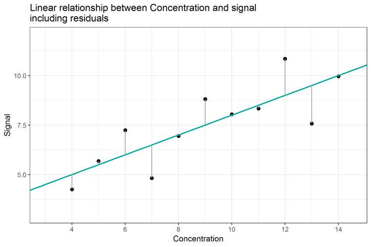
Figure 2: Linear Relationship between analyte concentration and signal, including residuals

As calculated in Table 1, the sum of all errors (the sum of residuals) is resulting in 0. This is because errors can positive or negative, as well – the model underestimates and overestimates. By summing up the errors, all errors compensate each other. This is a fundamental characteristic of the regression line and the method of least squares. Therefore, the sum of residuals can’t be used as an indicator of how well the regression line fits the data.

Table 1: Residuals X-values

x-values	4	5	6	7	8	9	10	11	12	13	14	Sum
Residuals	-0.740	0.179	1.239	-1.680	-0.050	1.309	0.039	-0.171	1.838	-1.921	-0.041	0

Since the sum of residuals is not an adequate measure to evaluate the validity of the regression model, we need to find another way to still use the residuals. To get rid of all negative values, we square the residuals (Table 2). This simple transformation has two advantages: First, the square of a number is always positive and as a consequence, each squared error cannot be negative anymore. Additionally, for small errors, e.g. errors less than 1 unit, the square of it will be even smaller and closer to 0 (e.g. 0.5² = 0.25). And for residuals bigger than 1, the squared residuals will be even bigger (e.g. 2.5² = 6.25). That means that small deviations from the regression line will be “rewarded”, while bigger deviations will be “penalized”.  

Table 2: X-values, residuals and squared residuals X-value

x-values	4	5	6	7	8	9	10	11	12	13	14	Sum
Residuals	-0.740	0.179	1.239	-1.680	-0.050	1.309	0.039	-0.171	1.838	-1.921	-0.041	0
Squared residuals	0.547	0.032	1.535	2.822	0.002	1.713	0.001	0.029	3.378	3.690	0.001	13754

Consequently, in a model with “larger” deviations, the sum of the squared residuals will be “larger” than in a model with “smaller” deviations. And therefore, we can use the sum of the squared residuals as a measure to evaluate model quality. As can be seen in Table 2, the sum of the squared residuals results in 13.75. This is actually the so-called residual sum of squares, or RSS. This is the value that the ICH Q2(R1) requires in method validation. It describes how much difference exists between the measured values and the ideal values of the regression line. Thus, small RSS values should always represent good mathematical models respectively calibration lines.

Now we know what the residual sum of squares is, but we still have not discussed the actual meaning of this measure. We know that smaller RSS might indicate a “better” model, or a “good” relationship between signal and concentration. But then, does this indicate that the method is fit-for-purpose? What is the threshold for the RSS? Or is there a threshold at all? In the ICH Q2(R1) guideline, there is no reference or comment regarding this aspect. It says that we need to state this number, but no interpretation of this number is needed. This is strange because the RSS is an indicator of model quality.

Since there is no RSS limit based on which we could declare the method as being fit-for-purpose, can we set a limit by ourselves? And if we are aiming for small RSS, could we just transform the data to decrease the RSS and make it look better? We could try by changing the units of the signal (Table 3). Let’s assume we would have a RSS value of 13.75, and the signal is given in Litres. What would happen if we use the exact same data, but transforming them to Gallons (1 Gallon = 4.54609 L)? What would happen to the regression line characteristics, and especially to the residual sum of squares?

Table 3: Differences in slope, y-intercept, RSS and R-squares, depending on signal units

	slope	y-intercept	RSS	R2
Litres	0.500	3.000	13.754	0.667
Gallons	0.109	0.660	0.666	0.667
Transformation	0.5 = 0.109 * 4.54609	3.0 = 0.66 * 4.54609	13.754 = 0.666 * 4.546092

The change of signal units would result in a change of regression characteristics, especially the slope, y-intercept and also in the residual sum of squares. Only, the R² value stays the same, which makes sense because there is still the same relationship between concentration and signal, it is independent of units. Astonishingly, the transformation results in a RSS of 0.666, a reduction of about 95% (!). That would sound much better in the validation report, wouldn’t it? ... having a RSS of less than 1 instead of more than 13.75...

And still, you cannot fool statistics because you can always back-transform the data using the factor of 4.54609, which will reveal the original values. Therefore, it doesn’t make sense to define any upper limit for the RSS because this characteristic depends on the method itself. It depends on the number of data points, e.g. on the number of replicates and concentrations, but also on the chosen values of concentrations. Thus, the RSS must always be considered together with the method itself, the R² and the characteristics of the regression line. Providing RSS without the other aspects is without any value. Therefore, it makes sense that the ICH Q2(R1) is requiring the RSS without any limit for the model. There cannot be a single limit for the RSS. As the RSS should always be regarded with all other data of the regression model, the following sentence of the guideline is absolutely warrantable:

“The … residual sum of squares should be submitted. A plot of the data should be included. In addition, an analysis of the deviation of the actual data points from the regression line may also be helpful for evaluating linearity.”

This sentence is of importance, even if the word may does not suggest that. Although the RSS gives us no hint whether the method satisfies any RSS condition, it could still happen that most of the data points contribute little to the overall RSS but one data point is far away from the regression line, such that its residual has a very big contribution to the overall RSS. Since the RSS equals the squared deviations from the regression line for all data points, we still do not know if there are some data points influencing the RSS more than others are doing. Therefore, it is suggested to further analyze the deviations and not only rely on the RSS itself.

If the method is fit-for-purpose, then the regression line should represent a physical or chemical relationship that exists between concentration and signal which, again, is dependent on the method itself. Therefore, the observed data points should also satisfy this relationship and we would not expect too large deviations from the physico-chemical relationship in our data. Each single data point should be close to this relationship and therefore close to the regression line. The RSS as a single measure cannot answer the question if one or more data points deviate too much from that relationship. To investigate the contribution of each data point to the RSS, we need to have a closer look into the data points and their deviation from the regression line. This might be the actual intention of the guideline: „analysis of the deviation of the actual data points from the regression line“.

 

From residual sum of squares back to single values

One idea to investigate the contribution of each data point is to measure its contribution by dividing its squared residual by the RSS. By doing so, we get a percentage of contribution and recognize that only 3 out of 14 data points (in bold) contribute about 70% to the total RSS. The data is summarized in Table 4:

Table 4: Contributions to the RSS by each data point

X-values	4	5	6	7	8	9	10	11	12	13	14	Sum
Residuals	-0.740	0.179	1.239	-1.680	-0.050	1.309	0.039	-0.171	1.838	-1.921	-0.041	0
Squared residuals	0.547	0.032	1.535	2.822	0.002	1.713	0.001	0.029	3.378	3.690	0.001	13754
Contribution (%)	3.98	0.23	11.16	20.52	0.01	12.45	0.01	0.21	24.56	26.82	0.01	100

 

 

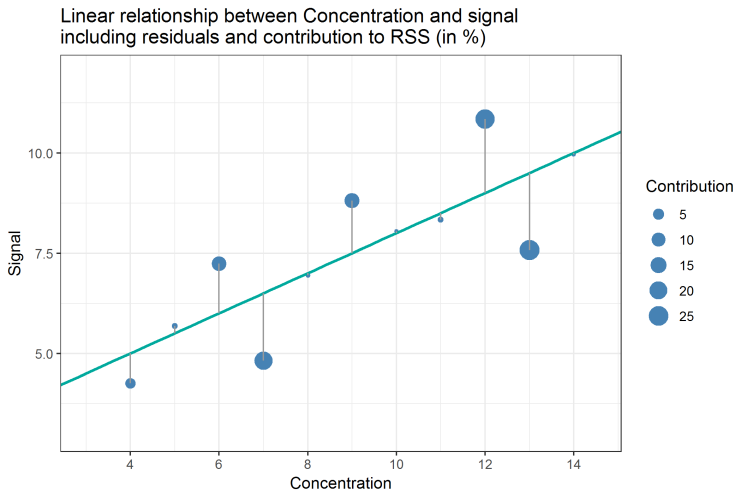
Figure 3: Linear Relationship between concentration and signal; size of data point corresponds to its contribution to RSS

We can also display the contribution of each data point by scaling the size of each data point according to its contribution (Figure 3). By doing so, we can at least visualize which data points contribute more than others. Now, which pattern of sizes would we expect as “normal” contributions? Again, using the percentages does not give us an exact answer to that. So, is there anything else we can do to find answers about that?

 

In the upcoming second part of this article, you'll learn how to examine the influence of each single data point, what Hat values and Cook's Distance are, and how to use Excel for such calculations.

 

About the author

Dr. Peter P. Heym wrote this article as guest author. He studied bioinformatics and obtained his PhD at the Leibnitz Institute for  Plant Biochemistry Halle with the topic "In silico characterisation of AtPARP1 and virtual screening for AtPARP inhibitors to increase resistance to abiotic stress". He is the CEO of Sum Of Squares - Statistical Consulting (www.sumofsquares.de), a service company specialized in statistical consulting for students, individuals, and companies. In addition to statistical advice he offers support for university thesis, evaluation of surveys, workshops (e.g. in programming language R), seminars, and trainings, also in GMP topics.